- AIA 15
- NuSTAR 10
- STIX 10
- XRT 7
- WCS 6
- spectroscopy 6
- STEREO 5
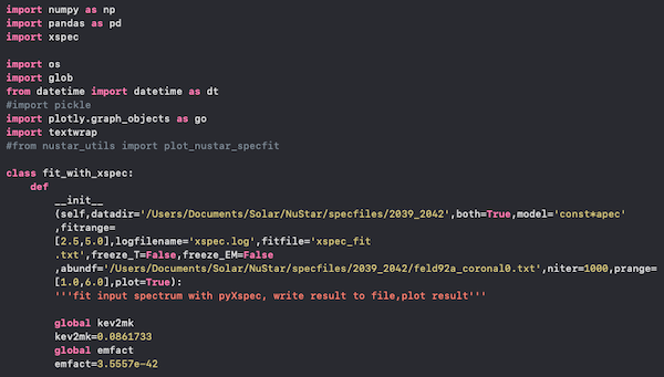
- xspec 4
- DEM 3
- computer vision 3
- deep learning 3
- examples 3
- visualization 3
- GOES 2
- PlotLy 2
- SPICE 2
- SunPy 2
- calculation 2
- HMI 1
- LLM 1
- MESSENGER 1
- MeerKAT 1
- figures 1
- image segmentation 1
- imaging 1
- published 1
AIA
Reprojecting STIX images
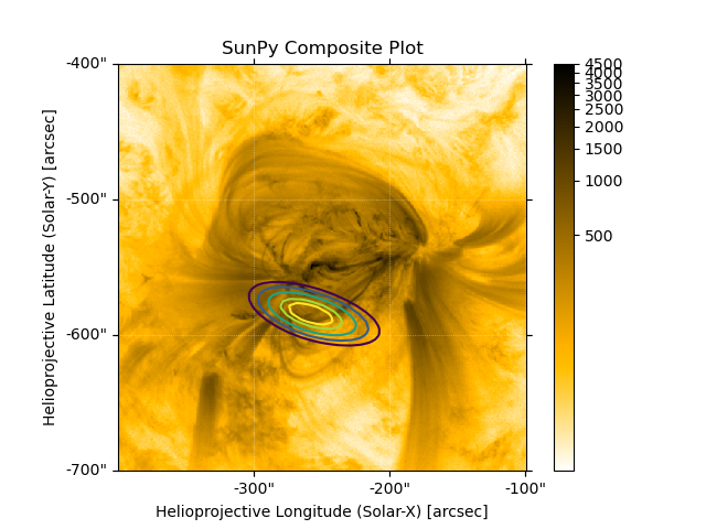
Previously, the reprojection of AIA maps to the Solar Orbiter reference frame has been shown. The method of reprojecting STIX images, reconstructed through one of many algorithms such as back projection, forward fit, CLEAN, or expectation maximization, is very similar.
DEXTR Image Segmentation test with HMI data
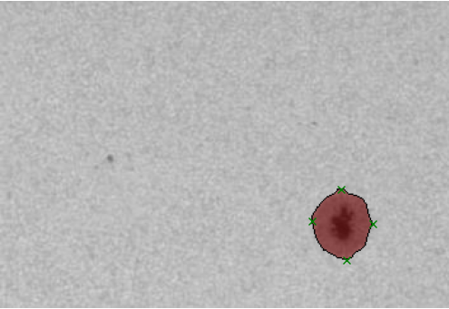
Deep Extreme Cut DEXTR uses extreme points of an object in an image as input to perform image segmentation. Here are some results of using the model trained on PASCAL VOC to segment HMI and AIA images (after conversion to RGB jpg).
Pre-trained model applied to HMI data
A faster way of reprojecting AIA cutouts
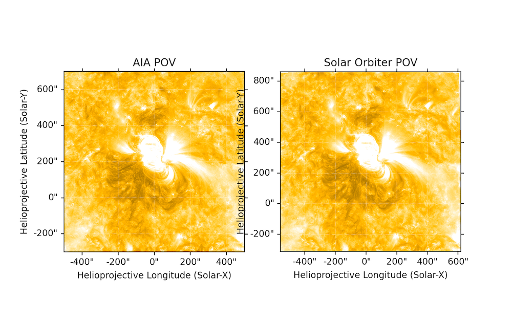
Reprojecting SunPy maps from one reference frame to another is most commonly done with full-disk images. The built-in implementation of reproject_to() is also capable of reprojecting submaps or cutouts; however, unless the output WCS are carefully adjusted this is just as slow as reprojecting a full-disk image.
Difference between SDO and Earth observers for coordinate rotation

The SPICE kernels used to get spacecraft or other oribiting body positions does not contain information for the SDO; therefore it is common to assume an Earth observer when considering coordinates associated with SDO/AIA data. Exact SDO location information is available through the FITS file headers. It’s inconvenient to download a large, fulldisk SDO image just to get its header, which is the way almost everyone knows how to access these keywords. There are lesser-known and/or used ways of getting header information alone, through dmrs or JSOC records queries.
Solar Orbiter flares visible by SDO

Solar Orbiter’s STIX has observed over 1000 flare candidates as of September 2021. Of those, 358 are given locations by the Coarse Flare Locator. Joint visibility with Earth-orbiting SDO can be determined using ephemeris information from Solar Orbiter, contained in the Spice kernels, and the Earth. Code is here.
DEMreg solutions - adding one wavelength at a time
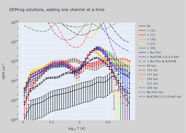
The shape of DEM solutions provided by DEMreg are strongly affected at high energies by the addition of Xray data. For completeness, I added each channel (both EUV and Xray) one at a time to the inputs to see how the solution was affected. The significant results are still what happens when the Xray data is added.
Sensitivity of DEMreg solutions to temperature range

The shape of joint DEM solutions (AIA + Xray) provided by DEMreg are very sensitive to the upper boundary of the selected temperature range.
AIA and NuSTAR loci curves
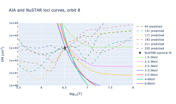
A quick check on appropriateness of spectral fits. Like with AIA, we can plot the NuSTAR loci curves, given here by the rate (counts s-1) divided by the appropriate temperature response (counts s-1 cm3) at a given energy. Select a variety of energies here in order to see which is most influential in contributing to the spectrum.
Calculating Expected AIA flux
To calculate expected flux (per AIA pixel) given a temperature and emission measure ( expected_AIA_flux() in flare_physics_utils.py):
NuSTAR small flare of 12 September 2020 - orbit 6 source 2
A second, much fainter source also close to the edge of the NuSTAR FOV examined with the initial intent of determining if the brighter source in the orbit left the FOV during the observation, thus accounting for the sudden drop in counts around 17:19.
NuSTAR small flare of 12 September 2020 - orbit 10
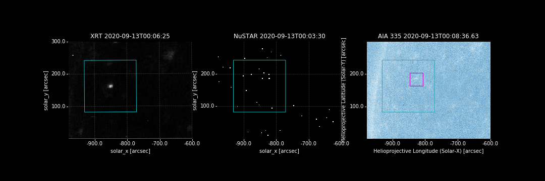
Basic information
NuSTAR small flare of 12 September 2020 - orbit 6
Basic information
NuSTAR small flare of 12 September 2020 - orbit 4

Basic information
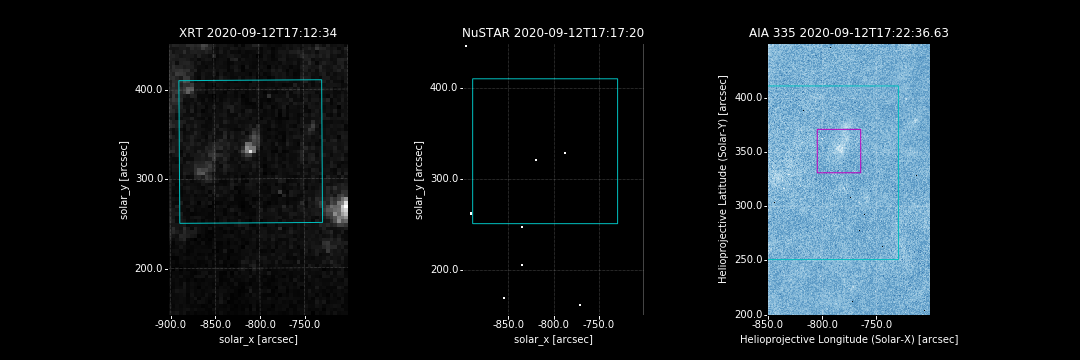
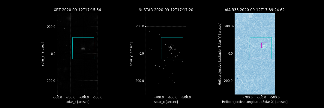
NuSTAR small flare of 12 September 2020 - orbit 8

Basic information
GOES-class Estimation for Behind-the-limb Solar Flares Using MESSENGER SAX
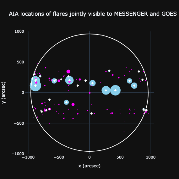
E. Lastufka (FHNW/ETHZ) and S. Krucker (FHNW/UC Berkeley)
NuSTAR
NuSTAR calibration update spectral fit comparison

Spectral fit
Fit to NuSTAR spectrum with pyXspec example
PyXspec is the Python interface to NASA’s X-ray Spectral Fitting Package.
DEMreg solutions - adding one wavelength at a time
The shape of DEM solutions provided by DEMreg are strongly affected at high energies by the addition of Xray data. For completeness, I added each channel (both EUV and Xray) one at a time to the inputs to see how the solution was affected. The significant results are still what happens when the Xray data is added.
Sensitivity of DEMreg solutions to temperature range
The shape of joint DEM solutions (AIA + Xray) provided by DEMreg are very sensitive to the upper boundary of the selected temperature range.
AIA and NuSTAR loci curves
A quick check on appropriateness of spectral fits. Like with AIA, we can plot the NuSTAR loci curves, given here by the rate (counts s-1) divided by the appropriate temperature response (counts s-1 cm3) at a given energy. Select a variety of energies here in order to see which is most influential in contributing to the spectrum.
NuSTAR small flare of 12 September 2020 - orbit 6 source 2
A second, much fainter source also close to the edge of the NuSTAR FOV examined with the initial intent of determining if the brighter source in the orbit left the FOV during the observation, thus accounting for the sudden drop in counts around 17:19.
NuSTAR small flare of 12 September 2020 - orbit 10
Basic information
NuSTAR small flare of 12 September 2020 - orbit 6
Basic information
NuSTAR small flare of 12 September 2020 - orbit 4
Basic information
NuSTAR small flare of 12 September 2020 - orbit 8
Basic information
STIX
GOES XRS daily background
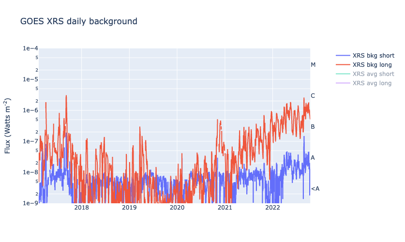
Daily X-ray background measurements are available for the last seven days at the Space Weather Prediction Center SWPC. The full dataset can be found here. No scaling factor is necessary for this data, as it is in physical units. To determine the daily background, hourly and 8-hour minima of the 1-minute averages are used. The 1-8 Å (long) and 0.5-4 Å (short) background fluxes are shown below, from February 2017 until October 2022. The daily average flux can also be toggled on.
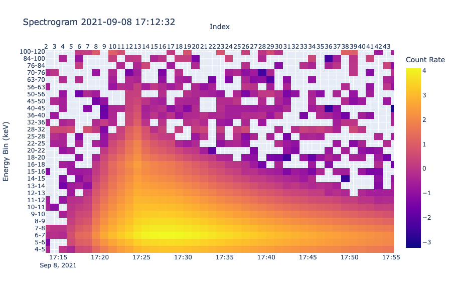
Cropping and Combining STIX spectrograms
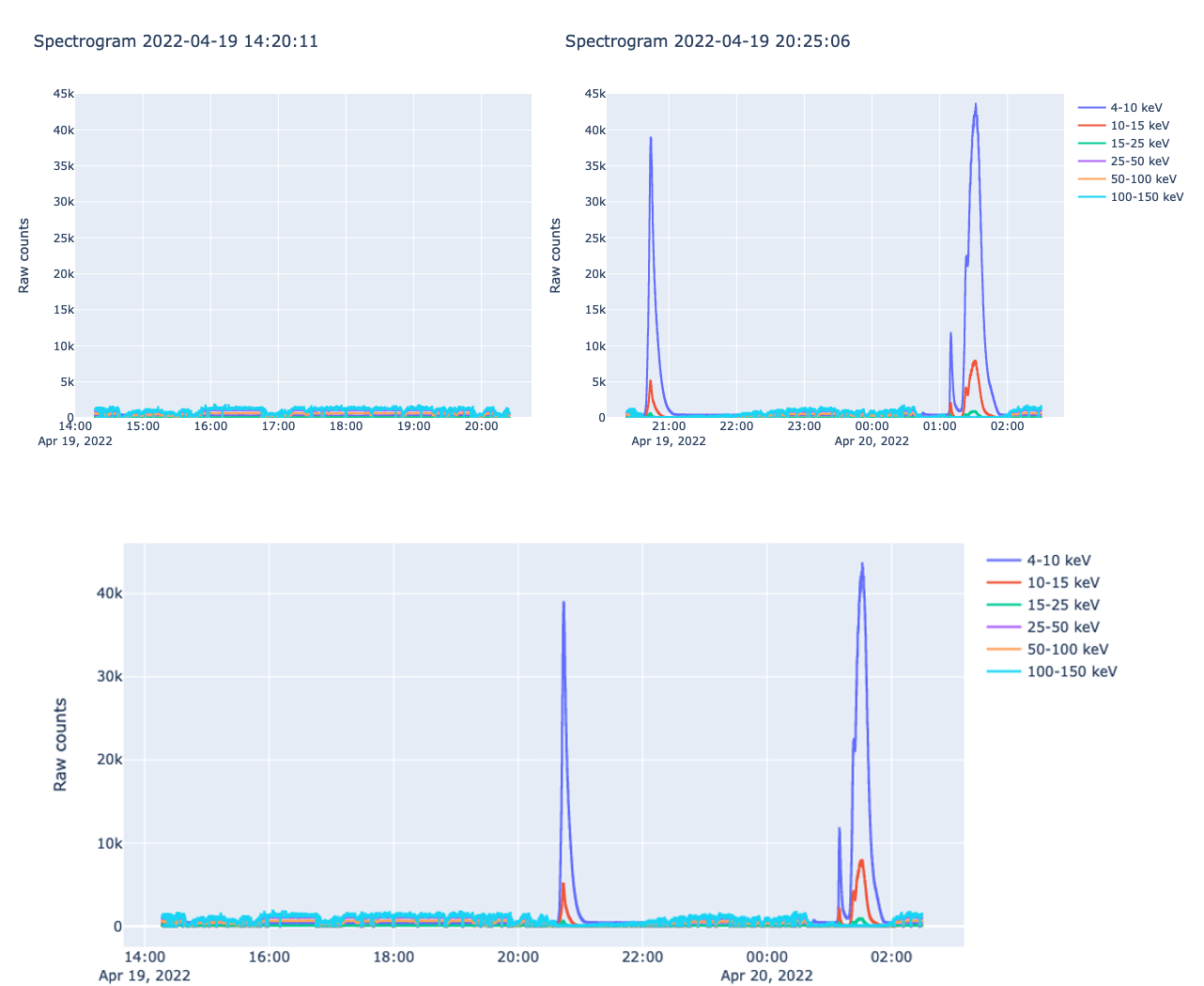
To select an event of interest from a long-duration spectrogram or pixel data file, one may want to reduce the file to a smaller size containing only that time period. Similarly, one might want to combine observations to cover a longer time period.
Back Projection to CLEAN Image Translation with Pix2Pix

Image-to-image translation has been sucessfully demonstrated for many cases, such as colorizing black-and-white images or filling in an object from its edges. Tensorflow has a detailed tutorial using Isola et al’s Pix2Pix. It uses a generator with a U-Net-based architecture and a discriminator using a convolutional PatchGAN classifier.
Reprojecting STIX images
Previously, the reprojection of AIA maps to the Solar Orbiter reference frame has been shown. The method of reprojecting STIX images, reconstructed through one of many algorithms such as back projection, forward fit, CLEAN, or expectation maximization, is very similar.
Thick Target Bremsstrahlung Model for XSPEC
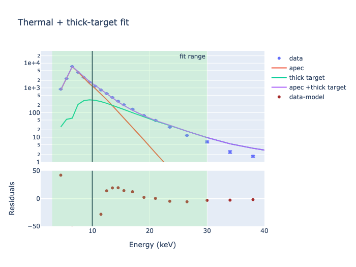
NASA’s X-ray Spectral Fitting Package lacks one of the key solar flare emission models, that of thick-target bremsstrahlung. In sswidl’s OSPEX, this model is implemented as thick2.pro. Using sunxspex’s emission module, the thick-target model can be adapted for use with XSPEC or PyXspec.
Fit to STIX spectrum with pyXspec
STIX spectrogram FITS files are not natively compatible with NASA’s X-ray Spectral Fitting Package. However, work is ongoing such that this powerful, free software can be used with STIX spectra, should sswidl’s OSPEX prove insufficient (ex., OSPEX can only fit with chi-squared minimization and one spectrum at a time).
A faster way of reprojecting AIA cutouts
Reprojecting SunPy maps from one reference frame to another is most commonly done with full-disk images. The built-in implementation of reproject_to() is also capable of reprojecting submaps or cutouts; however, unless the output WCS are carefully adjusted this is just as slow as reprojecting a full-disk image.
Spacecraft Roll Angle and Apparent Solar Radius from Spiceypy
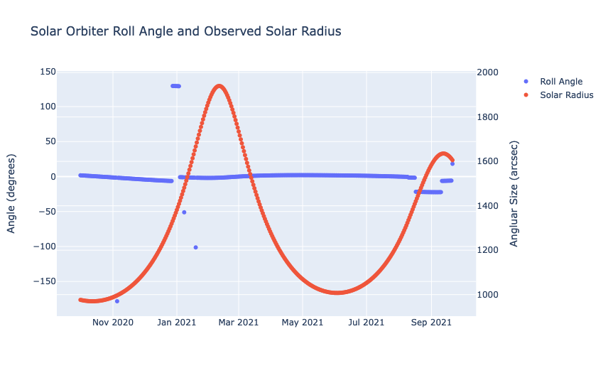
The as-flown attitude of an orbiting spacecraft affects its local coordinate system. A roll angle correction must be applied to imaging data in order to recover the proper coordinates. Spacecraft attitude data, both predicted and as-flown, are stored in the SPICE kernels.
Difference between SDO and Earth observers for coordinate rotation
The SPICE kernels used to get spacecraft or other oribiting body positions does not contain information for the SDO; therefore it is common to assume an Earth observer when considering coordinates associated with SDO/AIA data. Exact SDO location information is available through the FITS file headers. It’s inconvenient to download a large, fulldisk SDO image just to get its header, which is the way almost everyone knows how to access these keywords. There are lesser-known and/or used ways of getting header information alone, through dmrs or JSOC records queries.
Solar Orbiter flares visible by SDO
Solar Orbiter’s STIX has observed over 1000 flare candidates as of September 2021. Of those, 358 are given locations by the Coarse Flare Locator. Joint visibility with Earth-orbiting SDO can be determined using ephemeris information from Solar Orbiter, contained in the Spice kernels, and the Earth. Code is here.
XRT
DEMreg solutions - adding one wavelength at a time
The shape of DEM solutions provided by DEMreg are strongly affected at high energies by the addition of Xray data. For completeness, I added each channel (both EUV and Xray) one at a time to the inputs to see how the solution was affected. The significant results are still what happens when the Xray data is added.
Sensitivity of DEMreg solutions to temperature range
The shape of joint DEM solutions (AIA + Xray) provided by DEMreg are very sensitive to the upper boundary of the selected temperature range.
NuSTAR small flare of 12 September 2020 - orbit 6 source 2
A second, much fainter source also close to the edge of the NuSTAR FOV examined with the initial intent of determining if the brighter source in the orbit left the FOV during the observation, thus accounting for the sudden drop in counts around 17:19.
NuSTAR small flare of 12 September 2020 - orbit 10
Basic information
NuSTAR small flare of 12 September 2020 - orbit 6
Basic information
NuSTAR small flare of 12 September 2020 - orbit 4
Basic information
NuSTAR small flare of 12 September 2020 - orbit 8
Basic information
WCS
Reprojecting STIX images
Previously, the reprojection of AIA maps to the Solar Orbiter reference frame has been shown. The method of reprojecting STIX images, reconstructed through one of many algorithms such as back projection, forward fit, CLEAN, or expectation maximization, is very similar.
A faster way of reprojecting AIA cutouts
Reprojecting SunPy maps from one reference frame to another is most commonly done with full-disk images. The built-in implementation of reproject_to() is also capable of reprojecting submaps or cutouts; however, unless the output WCS are carefully adjusted this is just as slow as reprojecting a full-disk image.
Spacecraft Roll Angle and Apparent Solar Radius from Spiceypy
The as-flown attitude of an orbiting spacecraft affects its local coordinate system. A roll angle correction must be applied to imaging data in order to recover the proper coordinates. Spacecraft attitude data, both predicted and as-flown, are stored in the SPICE kernels.
Difference between SDO and Earth observers for coordinate rotation
The SPICE kernels used to get spacecraft or other oribiting body positions does not contain information for the SDO; therefore it is common to assume an Earth observer when considering coordinates associated with SDO/AIA data. Exact SDO location information is available through the FITS file headers. It’s inconvenient to download a large, fulldisk SDO image just to get its header, which is the way almost everyone knows how to access these keywords. There are lesser-known and/or used ways of getting header information alone, through dmrs or JSOC records queries.
Solar Orbiter flares visible by SDO
Solar Orbiter’s STIX has observed over 1000 flare candidates as of September 2021. Of those, 358 are given locations by the Coarse Flare Locator. Joint visibility with Earth-orbiting SDO can be determined using ephemeris information from Solar Orbiter, contained in the Spice kernels, and the Earth. Code is here.
Displaying SunPy maps with PlotLy
PlotLy lacks matplotlib’s projections function, which allows the user to add custom coordinates to their maps using transforms. In order to use solar maps in PlotLy and Dash, these transforms have to be applied (or faked!) elsewhere.
spectroscopy
GOES XRS daily background
Daily X-ray background measurements are available for the last seven days at the Space Weather Prediction Center SWPC. The full dataset can be found here. No scaling factor is necessary for this data, as it is in physical units. To determine the daily background, hourly and 8-hour minima of the 1-minute averages are used. The 1-8 Å (long) and 0.5-4 Å (short) background fluxes are shown below, from February 2017 until October 2022. The daily average flux can also be toggled on.
Cropping and Combining STIX spectrograms
To select an event of interest from a long-duration spectrogram or pixel data file, one may want to reduce the file to a smaller size containing only that time period. Similarly, one might want to combine observations to cover a longer time period.
Thick Target Bremsstrahlung Model for XSPEC
NASA’s X-ray Spectral Fitting Package lacks one of the key solar flare emission models, that of thick-target bremsstrahlung. In sswidl’s OSPEX, this model is implemented as thick2.pro. Using sunxspex’s emission module, the thick-target model can be adapted for use with XSPEC or PyXspec.
Fit to STIX spectrum with pyXspec
STIX spectrogram FITS files are not natively compatible with NASA’s X-ray Spectral Fitting Package. However, work is ongoing such that this powerful, free software can be used with STIX spectra, should sswidl’s OSPEX prove insufficient (ex., OSPEX can only fit with chi-squared minimization and one spectrum at a time).
NuSTAR calibration update spectral fit comparison
Spectral fit
Fit to NuSTAR spectrum with pyXspec example
PyXspec is the Python interface to NASA’s X-ray Spectral Fitting Package.
STEREO
NuSTAR small flare of 12 September 2020 - orbit 6 source 2
A second, much fainter source also close to the edge of the NuSTAR FOV examined with the initial intent of determining if the brighter source in the orbit left the FOV during the observation, thus accounting for the sudden drop in counts around 17:19.
NuSTAR small flare of 12 September 2020 - orbit 10
Basic information
NuSTAR small flare of 12 September 2020 - orbit 6
Basic information
NuSTAR small flare of 12 September 2020 - orbit 4
Basic information
NuSTAR small flare of 12 September 2020 - orbit 8
Basic information
xspec
Thick Target Bremsstrahlung Model for XSPEC
NASA’s X-ray Spectral Fitting Package lacks one of the key solar flare emission models, that of thick-target bremsstrahlung. In sswidl’s OSPEX, this model is implemented as thick2.pro. Using sunxspex’s emission module, the thick-target model can be adapted for use with XSPEC or PyXspec.
Fit to STIX spectrum with pyXspec
STIX spectrogram FITS files are not natively compatible with NASA’s X-ray Spectral Fitting Package. However, work is ongoing such that this powerful, free software can be used with STIX spectra, should sswidl’s OSPEX prove insufficient (ex., OSPEX can only fit with chi-squared minimization and one spectrum at a time).
NuSTAR calibration update spectral fit comparison
Spectral fit
Fit to NuSTAR spectrum with pyXspec example
PyXspec is the Python interface to NASA’s X-ray Spectral Fitting Package.
DEM
NuSTAR calibration update spectral fit comparison
Spectral fit
DEMreg solutions - adding one wavelength at a time
The shape of DEM solutions provided by DEMreg are strongly affected at high energies by the addition of Xray data. For completeness, I added each channel (both EUV and Xray) one at a time to the inputs to see how the solution was affected. The significant results are still what happens when the Xray data is added.
Sensitivity of DEMreg solutions to temperature range
The shape of joint DEM solutions (AIA + Xray) provided by DEMreg are very sensitive to the upper boundary of the selected temperature range.
computer vision
What Florence-2 thinks of the universe
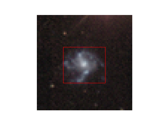
Florence-2 is a vision-language foundation model developed by Microsoft, designed to handle a variety of computer vision and vision-language tasks using a unified, prompt-based approach. It’s trained on a dataset that combines common image datasets like ImageNet with five billion annotations, and it seems to have some knowledge about astronomy. Here’s a few examples from optical, radio, and solar images, along with some very qualitative commentary.
Back Projection to CLEAN Image Translation with Pix2Pix
Image-to-image translation has been sucessfully demonstrated for many cases, such as colorizing black-and-white images or filling in an object from its edges. Tensorflow has a detailed tutorial using Isola et al’s Pix2Pix. It uses a generator with a U-Net-based architecture and a discriminator using a convolutional PatchGAN classifier.
DEXTR Image Segmentation test with HMI data
Deep Extreme Cut DEXTR uses extreme points of an object in an image as input to perform image segmentation. Here are some results of using the model trained on PASCAL VOC to segment HMI and AIA images (after conversion to RGB jpg).
Pre-trained model applied to HMI data
deep learning
What Florence-2 thinks of the universe
Florence-2 is a vision-language foundation model developed by Microsoft, designed to handle a variety of computer vision and vision-language tasks using a unified, prompt-based approach. It’s trained on a dataset that combines common image datasets like ImageNet with five billion annotations, and it seems to have some knowledge about astronomy. Here’s a few examples from optical, radio, and solar images, along with some very qualitative commentary.
Back Projection to CLEAN Image Translation with Pix2Pix
Image-to-image translation has been sucessfully demonstrated for many cases, such as colorizing black-and-white images or filling in an object from its edges. Tensorflow has a detailed tutorial using Isola et al’s Pix2Pix. It uses a generator with a U-Net-based architecture and a discriminator using a convolutional PatchGAN classifier.
DEXTR Image Segmentation test with HMI data
Deep Extreme Cut DEXTR uses extreme points of an object in an image as input to perform image segmentation. Here are some results of using the model trained on PASCAL VOC to segment HMI and AIA images (after conversion to RGB jpg).
Pre-trained model applied to HMI data
examples
Thick Target Bremsstrahlung Model for XSPEC
NASA’s X-ray Spectral Fitting Package lacks one of the key solar flare emission models, that of thick-target bremsstrahlung. In sswidl’s OSPEX, this model is implemented as thick2.pro. Using sunxspex’s emission module, the thick-target model can be adapted for use with XSPEC or PyXspec.
Fit to STIX spectrum with pyXspec
STIX spectrogram FITS files are not natively compatible with NASA’s X-ray Spectral Fitting Package. However, work is ongoing such that this powerful, free software can be used with STIX spectra, should sswidl’s OSPEX prove insufficient (ex., OSPEX can only fit with chi-squared minimization and one spectrum at a time).
Fit to NuSTAR spectrum with pyXspec example
PyXspec is the Python interface to NASA’s X-ray Spectral Fitting Package.
visualization
Reprojecting STIX images
Previously, the reprojection of AIA maps to the Solar Orbiter reference frame has been shown. The method of reprojecting STIX images, reconstructed through one of many algorithms such as back projection, forward fit, CLEAN, or expectation maximization, is very similar.
SunPy colormaps in PlotLy
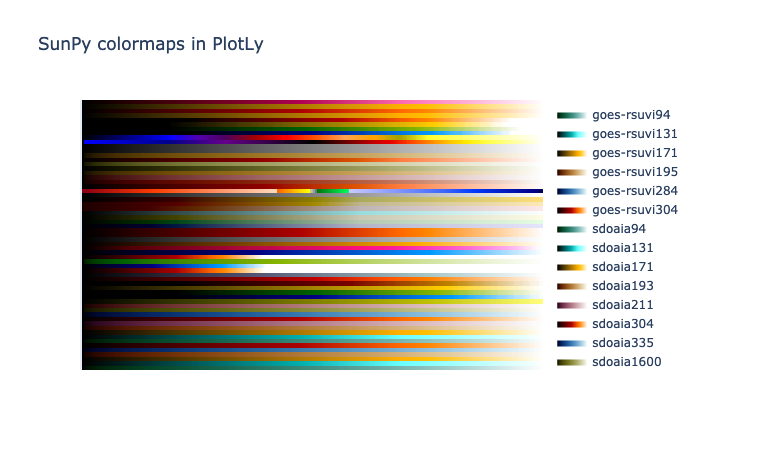
Solar image data has its own special set of colorscales associated with it. Certain instruments and wavelengths are by default presented in these scales, making their identification quick by the trained eye. SunPy has implemented most of these colormaps in its visualization.colormaps module. To use them in PlotLy, simply convert the LinearSegmentedColorscales to rgb values and add intervals to use them as PlotLy colorscales.
Displaying SunPy maps with PlotLy
PlotLy lacks matplotlib’s projections function, which allows the user to add custom coordinates to their maps using transforms. In order to use solar maps in PlotLy and Dash, these transforms have to be applied (or faked!) elsewhere.
GOES
GOES XRS daily background
Daily X-ray background measurements are available for the last seven days at the Space Weather Prediction Center SWPC. The full dataset can be found here. No scaling factor is necessary for this data, as it is in physical units. To determine the daily background, hourly and 8-hour minima of the 1-minute averages are used. The 1-8 Å (long) and 0.5-4 Å (short) background fluxes are shown below, from February 2017 until October 2022. The daily average flux can also be toggled on.
GOES-class Estimation for Behind-the-limb Solar Flares Using MESSENGER SAX
E. Lastufka (FHNW/ETHZ) and S. Krucker (FHNW/UC Berkeley)
PlotLy
SunPy colormaps in PlotLy
Solar image data has its own special set of colorscales associated with it. Certain instruments and wavelengths are by default presented in these scales, making their identification quick by the trained eye. SunPy has implemented most of these colormaps in its visualization.colormaps module. To use them in PlotLy, simply convert the LinearSegmentedColorscales to rgb values and add intervals to use them as PlotLy colorscales.
Displaying SunPy maps with PlotLy
PlotLy lacks matplotlib’s projections function, which allows the user to add custom coordinates to their maps using transforms. In order to use solar maps in PlotLy and Dash, these transforms have to be applied (or faked!) elsewhere.
SPICE
A faster way of reprojecting AIA cutouts
Reprojecting SunPy maps from one reference frame to another is most commonly done with full-disk images. The built-in implementation of reproject_to() is also capable of reprojecting submaps or cutouts; however, unless the output WCS are carefully adjusted this is just as slow as reprojecting a full-disk image.
Spacecraft Roll Angle and Apparent Solar Radius from Spiceypy
The as-flown attitude of an orbiting spacecraft affects its local coordinate system. A roll angle correction must be applied to imaging data in order to recover the proper coordinates. Spacecraft attitude data, both predicted and as-flown, are stored in the SPICE kernels.
SunPy
SunPy colormaps in PlotLy
Solar image data has its own special set of colorscales associated with it. Certain instruments and wavelengths are by default presented in these scales, making their identification quick by the trained eye. SunPy has implemented most of these colormaps in its visualization.colormaps module. To use them in PlotLy, simply convert the LinearSegmentedColorscales to rgb values and add intervals to use them as PlotLy colorscales.
Displaying SunPy maps with PlotLy
PlotLy lacks matplotlib’s projections function, which allows the user to add custom coordinates to their maps using transforms. In order to use solar maps in PlotLy and Dash, these transforms have to be applied (or faked!) elsewhere.
calculation
AIA and NuSTAR loci curves
A quick check on appropriateness of spectral fits. Like with AIA, we can plot the NuSTAR loci curves, given here by the rate (counts s-1) divided by the appropriate temperature response (counts s-1 cm3) at a given energy. Select a variety of energies here in order to see which is most influential in contributing to the spectrum.
Calculating Expected AIA flux
To calculate expected flux (per AIA pixel) given a temperature and emission measure ( expected_AIA_flux() in flare_physics_utils.py):
HMI
DEXTR Image Segmentation test with HMI data
Deep Extreme Cut DEXTR uses extreme points of an object in an image as input to perform image segmentation. Here are some results of using the model trained on PASCAL VOC to segment HMI and AIA images (after conversion to RGB jpg).
Pre-trained model applied to HMI data
LLM
What Florence-2 thinks of the universe
Florence-2 is a vision-language foundation model developed by Microsoft, designed to handle a variety of computer vision and vision-language tasks using a unified, prompt-based approach. It’s trained on a dataset that combines common image datasets like ImageNet with five billion annotations, and it seems to have some knowledge about astronomy. Here’s a few examples from optical, radio, and solar images, along with some very qualitative commentary.
MESSENGER
GOES-class Estimation for Behind-the-limb Solar Flares Using MESSENGER SAX
E. Lastufka (FHNW/ETHZ) and S. Krucker (FHNW/UC Berkeley)
MeerKAT
What Florence-2 thinks of the universe
Florence-2 is a vision-language foundation model developed by Microsoft, designed to handle a variety of computer vision and vision-language tasks using a unified, prompt-based approach. It’s trained on a dataset that combines common image datasets like ImageNet with five billion annotations, and it seems to have some knowledge about astronomy. Here’s a few examples from optical, radio, and solar images, along with some very qualitative commentary.
figures
GOES-class Estimation for Behind-the-limb Solar Flares Using MESSENGER SAX
E. Lastufka (FHNW/ETHZ) and S. Krucker (FHNW/UC Berkeley)
image segmentation
DEXTR Image Segmentation test with HMI data
Deep Extreme Cut DEXTR uses extreme points of an object in an image as input to perform image segmentation. Here are some results of using the model trained on PASCAL VOC to segment HMI and AIA images (after conversion to RGB jpg).
Pre-trained model applied to HMI data
imaging
Reprojecting STIX images
Previously, the reprojection of AIA maps to the Solar Orbiter reference frame has been shown. The method of reprojecting STIX images, reconstructed through one of many algorithms such as back projection, forward fit, CLEAN, or expectation maximization, is very similar.
published
GOES-class Estimation for Behind-the-limb Solar Flares Using MESSENGER SAX
E. Lastufka (FHNW/ETHZ) and S. Krucker (FHNW/UC Berkeley)